![[Photo of the Author]](../../common/images2/RalfWieland2.jpg)
original in de Ralf Wieland
de to en Jürgen Pohl
I am dealing with environment simulations, neural networks and fuzzy systems by programming them. The latter is being done under Linux ( since 0.99pl12). Furthermore, I am interested in electronics and in hardware, I am trying to relate that to Linux.
![[Illustration]](../../common/images2/article345/symbol.png)
I am working in a research
institute which is engaged in landscape research. Questions
like these are being investigated:
The daily legwork, consisting in analyzing of data, bitching about flawed measuring data, reformating of different data formats, writing of reports, etc., benefits tremendously from Linux. Even if some believe Excel and such can do everything, the combination of Perl, Emacs, octave [www.octave.org], R [www.r-project.org] etc. proves to be a strong contender in the battle with the data. Perl is very versatile, not limited to converting data; it queries data bases (MySQL), executes calculations, etc., fast and reproduceable. Specifically the latter is important since manual work frequently leads to mistakes in the data, this is rarely the case with the application of proven scripts. Writing articles with LaTeX convinces through its quality of appearance. Linux provides tools which make it attraktiv for scientific work. We do not want to conceal one disadvantage: one has to be intensely involved in utilizing those tools. Not everything can be done intuitively and not everyone is a programming freak.
Why has one to develop everything oneself, isn't it all
available? There are high-performance tools available for
simulations, like Matlab
[www.mathworks.com]. To process geographic data the
Geographic Information Systems (GIS) like ARCGIS
[www.esri.com/software/arcgis] or the free software Grass [grass.itc.it] are
available. For statistics it does not look much different. So,
why continuing to develop?
The problem is not the performance of the single components
but their collaboration in a system. In a simulation, subtasks
have to be performed by different programs, which may
communicate only cumbersomely, meaning through user-produced
interfaces. Aggravating is the fact, that the data available
are mass data (spatial data) with high error rates. The
essential simulations have to accommodate for this trait. An
algorithm has to supply useful results even when the data
entered do not fully match, a warning should be given in that
case. The processing of mass data (matrices with more then one
million elements are the rule) require fast algorithms. Robust
and fast algorithms can often be implemented only by developing
them by one's own.
The significant drawback of commercial systems is the secrecy
of the source codes. How can scientists develop and exchange
models if the sources are not open? From this conclusion it was
decided to develop a "Spatial Analysis and Modeling Tool"
(SAMT) as open source software.
It is a simulation tool, incorporating data management for
spatial data, interfaces to the MySQL data base and to GIS. It
contains fundamental functions for the management of raster
based data, it is able to manipulate rasters (blending,
distances, interpolation, etc.) and is able to generate a two
dimensional or three dimensional presentation of the data.
Note: raster data are based on dividing a map into a
small-square grid. The information is stored in several layers
of raster data. A model accesses the information of the layers.
Besides approaching the information in the depth, the
surrounding information on the same level are fundamental. The
latter are the basis for the modeling of lateral material
flows, as they occur in soil erosion, caused by wind and
water.
SAMT generates the framework into which the tools - like a
(very fast) fuzzy interpreter and the neural network tool
(nnqt) - may be adapted to. Fuzzy models serve to
integrate expert knowledge into the simulation. An expert can
often describe a process or even control it, even if no
mathematical model is available. Neural netsworks are processes
which allow us to derive functional correlations from measuring
data. The following shall introduce the development of the
neural network tool.
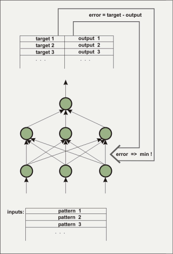
A artificial neural network consists of several layers. The first layer will be loaded with the initial data to be trained, in the form of floating-point numbers. The layer between input and output is not directly visible to the outside, it is called 'hidden layer'. Sometimes several hidden layers are present. The output layer of the example is only one element. This kind of architecture is used to build one function from several inputs and one output. The hidden layers are necessary to map non-linear behavior, for example the function x^2-y^2. How does a net know the wanted function? Initially, of course, the net does not know the function. The connections (weightings) between the elements (nodes) are attributed with stochastic values. During the training process the learnig algorithm tries to change the weightings in such a way that the mean square error between the computed and a predetermined output reaches a minimum. There are a variety of algorithms to accomplish this with, we are not going to elaborate on them here. Three algorithms were implemented into nnqt. Contingent on the input for the designated output, this process is also called 'supervised learning'.
The net is trained to detect if it has reached a small
enough error with the training data as well as the control data
(it is advisable to separate part of the data prior to the
training to use them as control data to verify the lerning
performance). The weightings determine the behaviour of the net
and they are being stored for that purpose. What is one able to
accomplish with such a net? In addition to the application as
modeling tool in science there are a number of more or less
serious applications. There are attempts to predict the trends
of the stock market. I was not successful with this, but maybe
someone else will do it.
Another interesting possibility would be the use of a neural
network for shorttime weatherforcasting. The data of electronic
weatherstations, for instance, could be used to train a neural
network. Useful would be the atmospheric pressure and its
changes, as well as the precipitation. The symbols on the
weatherstations follow these pattern. A neural net may do it
possibly better? To support one`s own experimentation
nnqt is available as GPL-software.
Scientists initiated the development of the neural network tool with their request that I may analyze their collected data. They wanted a tool as simple as possible, which should be able to be utilized for spatial applications, meaning: they whished to see how the results relate to the spatial placement. Of course, there are excellent neural network tools on the market. Even free tools like SNNS [www-ra.informatik.uni-tuebingen.de/SNNS/] or software libraries like fann [fann.sourceforge.net] are available. SNNS is great, but it is not easy to use for someone who is not able to program, since it delivers output in C-source code. In its scope it may be a bit overwhelming for the occasional user. nnqt had to meet a number of requirements:
The development took place in the following steps:
There is an overwhelming amount of good literature on neural
nets. As representative for most of it one book may be mentioned. However, sometimes there
is a gap which has to be closed through one's own
experimentation or by exchanges with others. I liked the fast
work with Matlab using the application of the
Levenberg-Marquardt-algorithm. Only after extensive internet
searches did I find an
articel
[www.eng.auburn.edu/~wilambm/pap/2001/FastConv_IJCNN01.PDF][local
copy, 105533 bytes] which describes this algorithm's use
for neural networks. That was the base. I had "only" the task
to integrate my favored tanh (tangens hyperbolicus)
functions into the algorithm. Also, for this I used Linux
software: the computer algebra system Maxima
[maxima.sourceforge.net]. It is possible with this kind of
system to manipulate complicated equations, to diffentiate and
so on, operations which are not so simple to solve with paper
and pencil. Maxima made it possible to perform the required
manipulations and to implement the first version of the
algorithm in C in a one-weekend session. The C-implementation
was done for testing and to tweak the parameters. By utilizing
the open source simulation system desire
[members.aol.com/gatmkorn] (many thanks to the developer
Prof. Korn!) as a tool for comparison, initial model
computations could be executed. The newly implemented algorithm
did not do too bad. The training time for the xor
problem, a favored test example for neural networks, achieved
an average of 70ms on a 3GHz Pentium computer. ( Much of this
time is being used by the reading operation of the harddrive,
the time on older Athlon 750MHz computers was slightly
higher).
As an alternative, the well known back propagation algorithm
was implemented and analyzed. After these preparations, which
are the basis for further improvements of the algorithms, the
implementation of the toolbox continued.
As a development environment I favor qt, it is well documented and I can use the Emacs editor. The qt designer assists with the design of the surface. Despite this the options are not sufficient for the development of nnqt. I needed something like diagrams, scales, etc. With this the developer community was again helpful. The libraries of qwt [qwt.sourceforge.net] and qwt3d [qwtplot3d.sourceforge.net] could be utilized, this helped to shorten the development time dramatically. Equipped with these sources, nnqt was built in about two weeks. When I was quite happy with the result, I turned to the users. They had many requests! The data set should be automatically divided into a training set and a test set, they wanted to be able to asign names to improve organization, more analysis - like graphs with parameter curves, etc. Well, some of it I was able to integrate immediately, other features will take a bit longer. Here are some screenshots:
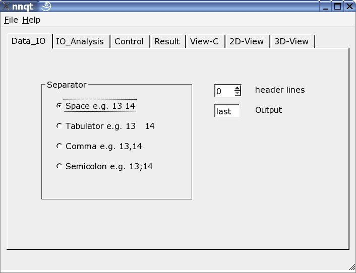
Here the reader can be adjusted to the input data format. Various separators may be used, some header lines may be hidden or the target in the data set may be freely chosen. Note: the data format should be known, since nnqt depends on the user input.
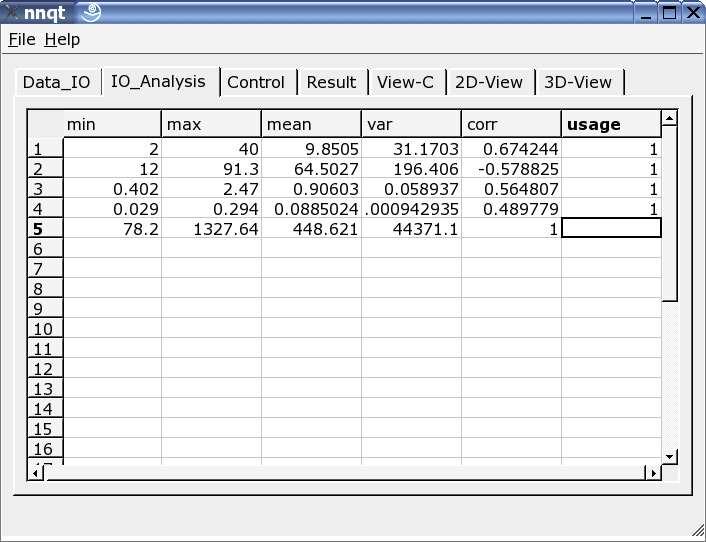
After successfully entering the data we are moving directly to the data analysis page. Here we are finding some information on the data, and the data for the training are to be selected from all the columns. A '1' in the last column marks the input as a training value. (Up to 29 training values may be utilized.)
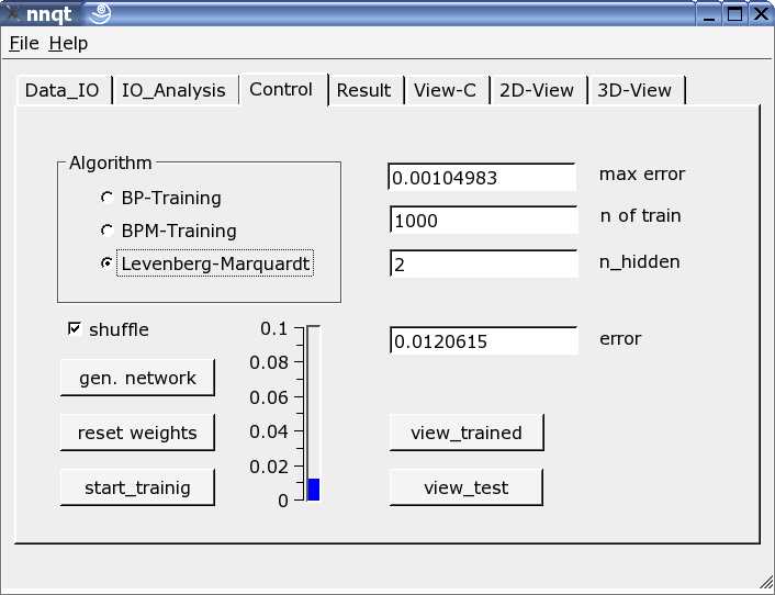
Most important is the control page. The number of hidden elements, the number of learning steps and the training algorithm are defined here. The training may be witnessed on the vertical scale as a bar and as a value. The training has to be repeated since the starting parameter was stochastically picked and the result is a direct function of it. Marking the check box "shuffle" generates a random selection - instead of a sequential selection - of the training data, which is sometimes advantageous. If we were successful with lowering the mean square error sufficiently, we may get the first graph by pushing the "view_trained" button:
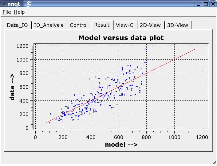
This shows the comparison of the trainings data with the data generated by the neural network. Ideally the data should be on the diagonal. But the ideal cannot be achieved! Nevertheless, the results look fairly decent. (The control data - they are the data which were not trained - are shown in red.) The next step allows the analysis of the function progression. The default values have to be set to meaningful numbers. With this we have to be careful, since the network's work reliably only close to the training data.
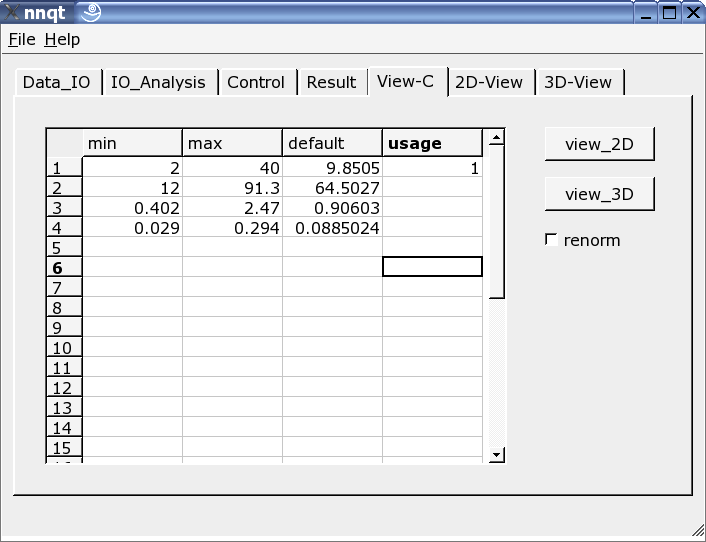
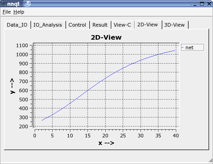
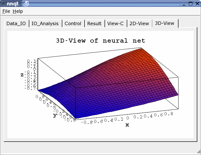
Two-dimensional or three-dimensional presentation may be chosen.
nnqt is open source software, it was released under
the GPL. Anyone can use it freely and improve it. The latter
would be especially great. The installation is quite simple.
Only the qwt libraries and qt must be installed.
nnqt.tgz is simple to unpack (tar-zxvf nnqt.tgz). This
will create a new directory named nnqt. Following a cd
nnqt, a qmake and a subsequent make will be
startet in the directory nnqt . If everything was interpreted
correctly a shell variable has to be set by executing:
export NN_HOME=/pfad_zu_nnqt
If nnqt is opened in a new terminal, the data and
models should be detected by nnqt. I hope you will have
a lot of fun with this. For the testing of the program a data
set with two inputs is included. Does someone recognize the
function which was lerned? ( it is x^2-y^2 in the range of
[-2..2].)
What could we create with all this - I am anxious to see your ideas.
It has been demonstrated, that Linux is an excellent development environment to solve scientific problems. I was able to do the development on the basis of excellent software, without that, it would have been impossible to create a usable tool in the short timespan of 6 weeks. It is always pleasant to be able to use free software. For this, many thanks to the many developers whose work made all the wonderful things possible we may do under Linux.
James A. Freeman:
"Simulating Neural Networks with Mathematica", Addison-Wesley
1994